Note
Click here to download the full example code
PyTorch Numeric Suite Tutorial
Introduction
Quantization is good when it works, but it’s difficult to know what’s wrong when it doesn’t satisfy the accuracy we expect. Debugging the accuracy issue of quantization is not easy and time consuming.
One important step of debugging is to measure the statistics of the float model and its corresponding quantized model to know where are they differ most. We built a suite of numeric tools called PyTorch Numeric Suite in PyTorch quantization to enable the measurement of the statistics between quantized module and float module to support quantization debugging efforts. Even for the quantized model with good accuracy, PyTorch Numeric Suite can still be used as the profiling tool to better understand the quantization error within the model and provide the guidance for further optimization.
PyTorch Numeric Suite currently supports models quantized through both static quantization and dynamic quantization with unified APIs.
In this tutorial we will first use ResNet18 as an example to show how to use PyTorch Numeric Suite to measure the statistics between static quantized model and float model in eager mode. Then we will use LSTM based sequence model as an example to show the usage of PyTorch Numeric Suite for dynamic quantized model.
Numeric Suite for Static Quantization
Setup
We’ll start by doing the necessary imports:
from __future__ import print_function, division, absolute_import
import numpy as np
import torch
import torch.nn as nn
import torchvision
from torchvision import datasets
import torchvision.transforms as transforms
import os
import torch.quantization
import torch.quantization._numeric_suite as ns
from torch.quantization import (
    default_eval_fn,
    default_qconfig,
    quantize,
)
Then we load the pretrained float ResNet18 model, and quantize it into qmodel. We cannot compare two arbitrary models, only a float model and the quantized model derived from it can be compared.
float_model = torchvision.models.quantization.resnet18(pretrained=True, quantize=False)
float_model.to('cpu')
float_model.eval()
float_model.fuse_model()
float_model.qconfig = torch.quantization.default_qconfig
img_data = [(torch.rand(2, 3, 10, 10, dtype=torch.float), torch.randint(0, 1, (2,), dtype=torch.long)) for _ in range(2)]
qmodel = quantize(float_model, default_eval_fn, [img_data], inplace=False)
1. Compare the weights of float and quantized models
The first thing we usually want to compare are the weights of quantized model and float model.
We can call compare_weights() from PyTorch Numeric Suite to get a dictionary wt_compare_dict with key corresponding to module names and each entry is a dictionary with two keys ‘float’ and ‘quantized’, containing the float and quantized weights.
compare_weights() takes in floating point and quantized state dict and returns a dict, with keys corresponding to the
floating point weights and values being a dictionary of floating point and quantized weights
wt_compare_dict = ns.compare_weights(float_model.state_dict(), qmodel.state_dict())

print('keys of wt_compare_dict:')
print(wt_compare_dict.keys())

print("\nkeys of wt_compare_dict entry for conv1's weight:")
print(wt_compare_dict['conv1.weight'].keys())
print(wt_compare_dict['conv1.weight']['float'].shape)
print(wt_compare_dict['conv1.weight']['quantized'].shape)
Out:
keys of wt_compare_dict:
dict_keys(['conv1.weight', 'layer1.0.conv1.weight', 'layer1.0.conv2.weight', 'layer1.1.conv1.weight', 'layer1.1.conv2.weight', 'layer2.0.conv1.weight', 'layer2.0.conv2.weight', 'layer2.0.downsample.0.weight', 'layer2.1.conv1.weight', 'layer2.1.conv2.weight', 'layer3.0.conv1.weight', 'layer3.0.conv2.weight', 'layer3.0.downsample.0.weight', 'layer3.1.conv1.weight', 'layer3.1.conv2.weight', 'layer4.0.conv1.weight', 'layer4.0.conv2.weight', 'layer4.0.downsample.0.weight', 'layer4.1.conv1.weight', 'layer4.1.conv2.weight', 'fc._packed_params._packed_params'])

keys of wt_compare_dict entry for conv1's weight:
dict_keys(['float', 'quantized'])
torch.Size([64, 3, 7, 7])
torch.Size([64, 3, 7, 7])
Once get wt_compare_dict, users can process this dictionary in whatever way they want. Here as an example we compute the quantization error of the weights of float and quantized models as following.
Compute the Signal-to-Quantization-Noise Ratio (SQNR) of the quantized tensor y. The SQNR reflects the
relationship between the maximum nominal signal strength and the quantization error introduced in the
quantization. Higher SQNR corresponds to lower quantization error.
def compute_error(x, y):
    Ps = torch.norm(x)
    Pn = torch.norm(x-y)
    return 20*torch.log10(Ps/Pn)

for key in wt_compare_dict:
    print(key, compute_error(wt_compare_dict[key]['float'], wt_compare_dict[key]['quantized'].dequantize()))
Out:
conv1.weight tensor(31.6638)
layer1.0.conv1.weight tensor(30.6450)
layer1.0.conv2.weight tensor(31.1528)
layer1.1.conv1.weight tensor(32.1438)
layer1.1.conv2.weight tensor(31.2477)
layer2.0.conv1.weight tensor(30.9890)
layer2.0.conv2.weight tensor(28.8233)
layer2.0.downsample.0.weight tensor(31.5558)
layer2.1.conv1.weight tensor(30.7668)
layer2.1.conv2.weight tensor(28.4515)
layer3.0.conv1.weight tensor(30.9246)
layer3.0.conv2.weight tensor(26.6839)
layer3.0.downsample.0.weight tensor(28.7825)
layer3.1.conv1.weight tensor(28.9705)
layer3.1.conv2.weight tensor(25.6781)
layer4.0.conv1.weight tensor(26.8492)
layer4.0.conv2.weight tensor(25.8381)
layer4.0.downsample.0.weight tensor(28.6355)
layer4.1.conv1.weight tensor(26.8749)
layer4.1.conv2.weight tensor(28.4311)
fc._packed_params._packed_params tensor(32.6504)
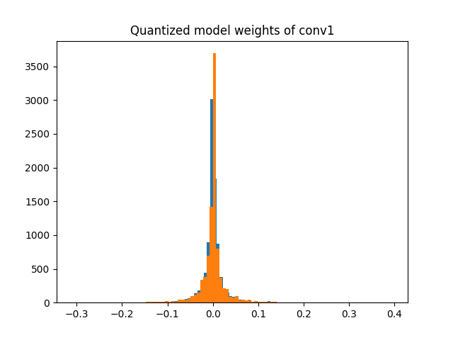
As another example wt_compare_dict can also be used to plot the histogram of the weights of floating point and quantized models.
import matplotlib.pyplot as plt

f = wt_compare_dict['conv1.weight']['float'].flatten()
plt.hist(f, bins = 100)
plt.title("Floating point model weights of conv1")
plt.show()

q = wt_compare_dict['conv1.weight']['quantized'].flatten().dequantize()
plt.hist(q, bins = 100)
plt.title("Quantized model weights of conv1")
plt.show()

2. Compare float point and quantized models at corresponding locations
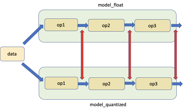
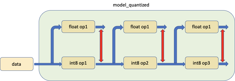
The second tool allows for comparison of weights and activations between float and quantized models at corresponding locations for the same input as shown in the figure below. Red arrows indicate the locations of the comparison.

We call compare_model_outputs() from PyTorch Numeric Suite to get the activations in float model and quantized model at corresponding locations for the given input data. This API returns a dict with module names being keys. Each entry is itself a dict with two keys ‘float’ and ‘quantized’ containing the activations.
data = img_data[0][0]

# Take in floating point and quantized model as well as input data, and returns a dict, with keys
# corresponding to the quantized module names and each entry being a dictionary with two keys 'float' and
# 'quantized', containing the activations of floating point and quantized model at matching locations.
act_compare_dict = ns.compare_model_outputs(float_model, qmodel, data)

print('keys of act_compare_dict:')
print(act_compare_dict.keys())

print("\nkeys of act_compare_dict entry for conv1's output:")
print(act_compare_dict['conv1.stats'].keys())
print(act_compare_dict['conv1.stats']['float'][0].shape)
print(act_compare_dict['conv1.stats']['quantized'][0].shape)
Out:
keys of act_compare_dict:
dict_keys(['conv1.stats', 'layer1.0.conv1.stats', 'layer1.0.conv2.stats', 'layer1.0.add_relu.stats', 'layer1.1.conv1.stats', 'layer1.1.conv2.stats', 'layer1.1.add_relu.stats', 'layer2.0.conv1.stats', 'layer2.0.conv2.stats', 'layer2.0.downsample.0.stats', 'layer2.0.add_relu.stats', 'layer2.1.conv1.stats', 'layer2.1.conv2.stats', 'layer2.1.add_relu.stats', 'layer3.0.conv1.stats', 'layer3.0.conv2.stats', 'layer3.0.downsample.0.stats', 'layer3.0.add_relu.stats', 'layer3.1.conv1.stats', 'layer3.1.conv2.stats', 'layer3.1.add_relu.stats', 'layer4.0.conv1.stats', 'layer4.0.conv2.stats', 'layer4.0.downsample.0.stats', 'layer4.0.add_relu.stats', 'layer4.1.conv1.stats', 'layer4.1.conv2.stats', 'layer4.1.add_relu.stats', 'fc.stats', 'quant.stats'])

keys of act_compare_dict entry for conv1's output:
dict_keys(['float', 'quantized'])
torch.Size([2, 64, 5, 5])
torch.Size([2, 64, 5, 5])
This dict can be used to compare and compute the quantization error of the activations of float and quantized models as following.
for key in act_compare_dict:
    print(key, compute_error(act_compare_dict[key]['float'][0], act_compare_dict[key]['quantized'][0].dequantize()))
Out:
conv1.stats tensor(37.4973, grad_fn=<MulBackward0>)
layer1.0.conv1.stats tensor(29.7153, grad_fn=<MulBackward0>)
layer1.0.conv2.stats tensor(28.5551, grad_fn=<MulBackward0>)
layer1.0.add_relu.stats tensor(32.1918, grad_fn=<MulBackward0>)
layer1.1.conv1.stats tensor(29.6006, grad_fn=<MulBackward0>)
layer1.1.conv2.stats tensor(25.4115, grad_fn=<MulBackward0>)
layer1.1.add_relu.stats tensor(29.0712, grad_fn=<MulBackward0>)
layer2.0.conv1.stats tensor(25.9490, grad_fn=<MulBackward0>)
layer2.0.conv2.stats tensor(26.0952, grad_fn=<MulBackward0>)
layer2.0.downsample.0.stats tensor(22.3922, grad_fn=<MulBackward0>)
layer2.0.add_relu.stats tensor(25.6427, grad_fn=<MulBackward0>)
layer2.1.conv1.stats tensor(25.1334, grad_fn=<MulBackward0>)
layer2.1.conv2.stats tensor(24.2990, grad_fn=<MulBackward0>)
layer2.1.add_relu.stats tensor(26.0615, grad_fn=<MulBackward0>)
layer3.0.conv1.stats tensor(26.9766, grad_fn=<MulBackward0>)
layer3.0.conv2.stats tensor(27.1612, grad_fn=<MulBackward0>)
layer3.0.downsample.0.stats tensor(25.3592, grad_fn=<MulBackward0>)
layer3.0.add_relu.stats tensor(25.5589, grad_fn=<MulBackward0>)
layer3.1.conv1.stats tensor(31.5189, grad_fn=<MulBackward0>)
layer3.1.conv2.stats tensor(26.1545, grad_fn=<MulBackward0>)
layer3.1.add_relu.stats tensor(25.6128, grad_fn=<MulBackward0>)
layer4.0.conv1.stats tensor(27.7432, grad_fn=<MulBackward0>)
layer4.0.conv2.stats tensor(27.3511, grad_fn=<MulBackward0>)
layer4.0.downsample.0.stats tensor(21.8674, grad_fn=<MulBackward0>)
layer4.0.add_relu.stats tensor(20.8096, grad_fn=<MulBackward0>)
layer4.1.conv1.stats tensor(25.5999, grad_fn=<MulBackward0>)
layer4.1.conv2.stats tensor(18.1554, grad_fn=<MulBackward0>)
layer4.1.add_relu.stats tensor(18.3537, grad_fn=<MulBackward0>)
fc.stats tensor(20.6431, grad_fn=<MulBackward0>)
quant.stats tensor(47.9820)
If we want to do the comparison for more than one input data, we can do the following.
Prepare the model by attaching the logger to both floating point module and quantized
module if they are in the white_list. Default logger is OutputLogger, and default white_list
is DEFAULT_NUMERIC_SUITE_COMPARE_MODEL_OUTPUT_WHITE_LIST
ns.prepare_model_outputs(float_model, qmodel)

for data in img_data:
    float_model(data[0])
    qmodel(data[0])

# Find the matching activation between floating point and quantized modules, and return a dict with key
# corresponding to quantized module names and each entry being a dictionary with two keys 'float'
# and 'quantized', containing the matching floating point and quantized activations logged by the logger
act_compare_dict = ns.get_matching_activations(float_model, qmodel)
The default logger used in above APIs is OutputLogger, which is used to log the outputs of the modules. We can inherit from base Logger class and create our own logger to perform different functionalities. For example we can make a new MyOutputLogger class as below.
class MyOutputLogger(ns.Logger):
    r"""Customized logger class
    """

    def __init__(self):
        super(MyOutputLogger, self).__init__()

    def forward(self, x):
        # Custom functionalities
        # ...
        return x
And then we can pass this logger into above APIs such as:
data = img_data[0][0]
act_compare_dict = ns.compare_model_outputs(float_model, qmodel, data, logger_cls=MyOutputLogger)
or:
ns.prepare_model_outputs(float_model, qmodel, MyOutputLogger)
for data in img_data:
    float_model(data[0])
    qmodel(data[0])
act_compare_dict = ns.get_matching_activations(float_model, qmodel)
3. Compare a module in a quantized model with its float point equivalent, with the same input data
The third tool allows for comparing a quantized module in a model with its float point counterpart, feeding both of them the same input and comparing their outputs as shown below.

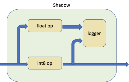
In practice we call prepare_model_with_stubs() to swap the quantized module that we want to compare with the Shadow module, which is illustrated as below:

The Shadow module takes quantized module, float module and logger as input, and creates a forward path inside to make the float module to shadow quantized module sharing the same input tensor.
The logger can be customizable, default logger is ShadowLogger and it will save the outputs of the quantized module and float module that can be used to compute the module level quantization error.
Notice before each call of compare_model_outputs() and compare_model_stub() we need to have clean float and quantized model. This is because compare_model_outputs() and compare_model_stub() modify float and quantized model inplace, and it will cause unexpected results if call one right after another.
float_model = torchvision.models.quantization.resnet18(pretrained=True, quantize=False)
float_model.to('cpu')
float_model.eval()
float_model.fuse_model()
float_model.qconfig = torch.quantization.default_qconfig
img_data = [(torch.rand(2, 3, 10, 10, dtype=torch.float), torch.randint(0, 1, (2,), dtype=torch.long)) for _ in range(2)]
qmodel = quantize(float_model, default_eval_fn, [img_data], inplace=False)
In the following example we call compare_model_stub() from PyTorch Numeric Suite to compare QuantizableBasicBlock module with its float point equivalent. This API returns a dict with key corresponding to module names and each entry being a dictionary with two keys ‘float’ and ‘quantized’, containing the output tensors of quantized and its matching float shadow module.
data = img_data[0][0]
module_swap_list = [torchvision.models.quantization.resnet.QuantizableBasicBlock]

# Takes in floating point and quantized model as well as input data, and returns a dict with key
# corresponding to module names and each entry being a dictionary with two keys 'float' and
# 'quantized', containing the output tensors of quantized module and its matching floating point shadow module.
ob_dict = ns.compare_model_stub(float_model, qmodel, module_swap_list, data)

print('keys of ob_dict:')
print(ob_dict.keys())

print("\nkeys of ob_dict entry for layer1.0's output:")
print(ob_dict['layer1.0.stats'].keys())
print(ob_dict['layer1.0.stats']['float'][0].shape)
print(ob_dict['layer1.0.stats']['quantized'][0].shape)
Out:
keys of ob_dict:
dict_keys(['layer1.0.stats', 'layer1.1.stats', 'layer2.0.stats', 'layer2.1.stats', 'layer3.0.stats', 'layer3.1.stats', 'layer4.0.stats', 'layer4.1.stats'])

keys of ob_dict entry for layer1.0's output:
dict_keys(['float', 'quantized'])
torch.Size([64, 3, 3])
torch.Size([64, 3, 3])
This dict can be then used to compare and compute the module level quantization error.
for key in ob_dict:
    print(key, compute_error(ob_dict[key]['float'][0], ob_dict[key]['quantized'][0].dequantize()))
Out:
layer1.0.stats tensor(32.4555)
layer1.1.stats tensor(33.3692)
layer2.0.stats tensor(29.1197)
layer2.1.stats tensor(31.3616)
layer3.0.stats tensor(28.9080)
layer3.1.stats tensor(31.8462)
layer4.0.stats tensor(25.1721)
layer4.1.stats tensor(22.7233)
If we want to do the comparison for more than one input data, we can do the following.
ns.prepare_model_with_stubs(float_model, qmodel, module_swap_list, ns.ShadowLogger)
for data in img_data:
    qmodel(data[0])
ob_dict = ns.get_logger_dict(qmodel)
The default logger used in above APIs is ShadowLogger, which is used to log the outputs of the quantized module and its matching float shadow module. We can inherit from base Logger class and create our own logger to perform different functionalities. For example we can make a new MyShadowLogger class as below.
class MyShadowLogger(ns.Logger):
    r"""Customized logger class
    """

    def __init__(self):
        super(MyShadowLogger, self).__init__()

    def forward(self, x, y):
        # Custom functionalities
        # ...
        return x
And then we can pass this logger into above APIs such as:
data = img_data[0][0]
ob_dict = ns.compare_model_stub(float_model, qmodel, module_swap_list, data, logger_cls=MyShadowLogger)
or:
ns.prepare_model_with_stubs(float_model, qmodel, module_swap_list, MyShadowLogger)
for data in img_data:
    qmodel(data[0])
ob_dict = ns.get_logger_dict(qmodel)
Numeric Suite for Dynamic Quantization
Numeric Suite APIs are designed in such as way that they work for both dynamic quantized model and static quantized model. We will use a model with both LSTM and Linear modules to demonstrate the usage of Numeric Suite on dynamic quantized model. This model is the same one used in the tutorial of dynamic quantization on LSTM word language model [1].
Setup
First we define the model as below. Notice that within this model only nn.LSTM and nn.Linear modules will be quantized dynamically and nn.Embedding will remain as floating point module after quantization.
class LSTMModel(nn.Module):
    """Container module with an encoder, a recurrent module, and a decoder."""

    def __init__(self, ntoken, ninp, nhid, nlayers, dropout=0.5):
        super(LSTMModel, self).__init__()
        self.encoder = nn.Embedding(ntoken, ninp)
        self.rnn = nn.LSTM(ninp, nhid, nlayers, dropout=dropout)
        self.decoder = nn.Linear(nhid, ntoken)

        self.init_weights()

        self.nhid = nhid
        self.nlayers = nlayers

    def init_weights(self):
        initrange = 0.1
        self.encoder.weight.data.uniform_(-initrange, initrange)
        self.decoder.bias.data.zero_()
        self.decoder.weight.data.uniform_(-initrange, initrange)

    def forward(self, input, hidden):
        emb = self.encoder(input)
        output, hidden = self.rnn(emb, hidden)
        decoded = self.decoder(output)
        return decoded, hidden

    def init_hidden(self, bsz):
        weight = next(self.parameters())
        return (weight.new_zeros(self.nlayers, bsz, self.nhid),
                weight.new_zeros(self.nlayers, bsz, self.nhid))
Then we create the float_model and quantize it into qmodel.
ntokens = 10

float_model = LSTMModel(
    ntoken = ntokens,
    ninp = 512,
    nhid = 256,
    nlayers = 5,
)

float_model.eval()

qmodel = torch.quantization.quantize_dynamic(
    float_model, {nn.LSTM, nn.Linear}, dtype=torch.qint8
)
1. Compare the weights of float and quantized models
We first call compare_weights() from PyTorch Numeric Suite to get a dictionary wt_compare_dict with key corresponding to module names and each entry is a dictionary with two keys ‘float’ and ‘quantized’, containing the float and quantized weights.
wt_compare_dict = ns.compare_weights(float_model.state_dict(), qmodel.state_dict())
Once we get wt_compare_dict, it can be used to compare and compute the quantization error of the weights of float and quantized models as following.
for key in wt_compare_dict:
    if wt_compare_dict[key]['quantized'].is_quantized:
        print(key, compute_error(wt_compare_dict[key]['float'], wt_compare_dict[key]['quantized'].dequantize()))
    else:
        print(key, compute_error(wt_compare_dict[key]['float'], wt_compare_dict[key]['quantized']))
Out:
encoder.weight tensor(inf)
rnn._all_weight_values.0.param tensor(48.1291)
rnn._all_weight_values.1.param tensor(48.1302)
rnn._all_weight_values.2.param tensor(48.1361)
rnn._all_weight_values.3.param tensor(48.1155)
rnn._all_weight_values.4.param tensor(48.1254)
decoder._packed_params._packed_params tensor(48.1111)
The Inf value in encoder.weight entry above is because encoder module is not quantized and the weights are the same in both floating point and quantized models.
2. Compare float point and quantized models at corresponding locations
Then we call compare_model_outputs() from PyTorch Numeric Suite to get the activations in float model and quantized model at corresponding locations for the given input data. This API returns a dict with module names being keys. Each entry is itself a dict with two keys ‘float’ and ‘quantized’ containing the activations. Notice that this sequence model has two inputs, and we can pass both inputs into compare_model_outputs() and compare_model_stub().
input_ = torch.randint(ntokens, (1, 1), dtype=torch.long)
hidden = float_model.init_hidden(1)

act_compare_dict = ns.compare_model_outputs(float_model, qmodel, input_, hidden)
print(act_compare_dict.keys())
Out:
dict_keys(['encoder.stats', 'rnn.stats', 'decoder.stats'])
This dict can be used to compare and compute the quantization error of the activations of float and quantized models as following. The LSTM module in this model has two outputs, in this example we compute the error of the first output.
for key in act_compare_dict:
    print(key, compute_error(act_compare_dict[key]['float'][0][0], act_compare_dict[key]['quantized'][0][0]))
Out:
encoder.stats tensor(inf, grad_fn=<MulBackward0>)
rnn.stats tensor(54.5561, grad_fn=<MulBackward0>)
decoder.stats tensor(36.1568, grad_fn=<MulBackward0>)
3. Compare a module in a quantized model with its float point equivalent, with the same input data
Next we call compare_model_stub() from PyTorch Numeric Suite to compare LSTM and Linear module with its float point equivalent. This API returns a dict with key corresponding to module names and each entry being a dictionary with two keys ‘float’ and ‘quantized’, containing the output tensors of quantized and its matching float shadow module.
We reset the model first.
float_model = LSTMModel(
    ntoken = ntokens,
    ninp = 512,
    nhid = 256,
    nlayers = 5,
)
float_model.eval()

qmodel = torch.quantization.quantize_dynamic(
    float_model, {nn.LSTM, nn.Linear}, dtype=torch.qint8
)
Next we call compare_model_stub() from PyTorch Numeric Suite to compare LSTM and Linear module with its float point equivalent. This API returns a dict with key corresponding to module names and each entry being a dictionary with two keys ‘float’ and ‘quantized’, containing the output tensors of quantized and its matching float shadow module.
module_swap_list = [nn.Linear, nn.LSTM]
ob_dict = ns.compare_model_stub(float_model, qmodel, module_swap_list, input_, hidden)
print(ob_dict.keys())
Out:
dict_keys(['rnn.stats', 'decoder.stats'])
This dict can be then used to compare and compute the module level quantization error.
for key in ob_dict:
    print(key, compute_error(ob_dict[key]['float'][0], ob_dict[key]['quantized'][0]))
Out:
rnn.stats tensor(55.7612)
decoder.stats tensor(37.4199)
SQNR of 40 dB is high and this is a situation where we have very good numerical alignment between the floating point and quantized model.
Conclusion
In this tutorial, we demonstrated how to use PyTorch Numeric Suite to measure and compare the statistics between quantized model and float model in eager mode with unified APIs for both static quantization and dynamic quantization.
Thanks for reading! As always, we welcome any feedback, so please create an issue here if you have any.
References
[1] DYNAMIC QUANTIZATION ON AN LSTM WORD LANGUAGE MODEL.
Total running time of the script: ( 0 minutes 4.895 seconds)


